Printing to pdf from Matlab via eps

I use pdflatex for my publications, both because it is convenient to have PDF as the output format, and also because it accepts many kinds of graphic files, like JPG and PNG. If you want to use a vector graphics format, then you can save your graphics as PDFs. This is quite easy to do in Matlab, but I have found that it often leads to rasterization artifacts in the graphics. Exporting to EPS seems to work a lot better in this regard. The solution: Exporting from Matlab in EPS format, and postconverting to PDF using the esptopdf function (part of the texlive-extra-utils). I have made a Matlab function to automate the process:

function printpdfviaeps(filename, varargin)
%PRINTPDFVIAEPS Print current figure to pdf via eps
%
% printpdfviaeps(filename) will save the current figure to filename.pdf,
% using a default paper size of width = 12 cm, height = 9 cm.
%
% printpdfviaeps(filename, width, height) lets you specify the width and
% height yourself.
%
% Martin Skjelvareid, 2010-11-11

width = 12; % Default width in centimeters
height = 9; % Default height in centimeters

if nargin > 1
width = varargin{1};
end
if nargin > 2
height = varargin{2};
end

set(gcf, 'PaperUnits', 'centimeters');
set(gcf, 'PaperSize', [width height]);
set(gcf, 'PaperPositionMode', 'manual');
set(gcf, 'PaperPosition', [0 0 width height]);

print('-deps2','-r150', filename)
system(['epstopdf ' filename '.eps']);
delete([filename '.eps'])

Resetting ssh server host key

Today I tried logging on to a server that was recently down due to a brute force attack. Using the SSH command resulted in the following warning:

@@@@@@@@@@@@@@@@@@@@@@@@@@@@@@@@@@@@@@@@@@@@@@@@@@@@@@@@@@@
@ WARNING: REMOTE HOST IDENTIFICATION HAS CHANGED! @
@@@@@@@@@@@@@@@@@@@@@@@@@@@@@@@@@@@@@@@@@@@@@@@@@@@@@@@@@@@
IT IS POSSIBLE THAT SOMEONE IS DOING SOMETHING NASTY!
Someone could be eavesdropping on you right now (man-in-the-middle attack)!
It is also possible that the RSA host key has just been changed.
[...]

In this case, the problem was that the RSA host key had changed. After searching the net for a while, I found that some people routinely delete their known_hosts file because of this. However, there is a proper solution to the problem, as presemted by *ccm* in this blog post:

ssh-keygen -R

where is replaced with the name of the server that you're trying to connect to.

Checking which memory banks are used on Linux

Today, I decided that I want to upgrade from 2 GB to 4 BG memory on my laptop. However, I didn't know how this memory was distributed - was it two 1GB chips, or a single 2 GB chip? Luckily, a colleague of mine found this command:

sudo lshw -c memory

which, among other things, produced these lines:

*-memory
description: System Memory
physical id: 2b
slot: System board or motherboard
size: 2GiB
*-bank:0
description: SODIMM DDR2 Synchronous 667 MHz (1.5 ns)
physical id: 0
slot: DIMM 1
size: 2GiB
width: 64 bits
clock: 667MHz (1.5ns)
*-bank:1
description: SODIMM DDR2 Synchronous 667 MHz (1.5 ns) [empty]
physical id: 1
slot: DIMM 2
clock: 667MHz (1.5ns)

Voila! From this info it's easy to see that memory bank 1 has 2 GB of memory, and bank 2 is empty.

Solving installation problems with Comsol 4.0a in Ubuntu Linux

Today I decided to install Comsol Multiphysics 4.0a, which is a physics simulation program based on the Finite Element Method (FEM). I'm running Ubuntu Linux 9.10 (Karmic Koala), and the installation procedure should be as simple as this (quoting from the installation manual):

"To start the installation, type the command

sh {drive path}/setup

where {drive path} refers to the mount point of the DVD-ROM
drive on your system, for example, /media/cdrom."

When I insterted the Comsol DVD, it was mounted as "COMSOL40a ". Note that there are some trailing white spaces which don't make any sense. When I tried to run the installation program, I got an error message saying that "/media/COMSOL40a" did not exist. Turns out that the installation program was looking for a mount point directory without any white spaces.

My solution to this was to mount the CD to another folder, to a folder name without trailing white spaces. I didn't know how do this, but I found a simple description at this web site. In the terminal, I typed

sudo mount -t auto /dev/cdrom /media/tmpcd/

to mount the CD to /media/tmpcd. After that, I could run the installation program as instructed, by typing

sh /media/tmpcd/setup

I'm not sure who is to blame for this "bug", Ubuntu or Comsol, but at least I figured out how to work around it. :-)

Solving Ubuntu full disk problem related to SBackup

OK, so today I came to my office finding that somehow my Wubi Ubuntu installation had somehow filled up completely. There was absolutely no disk space left, and because of this, the whole system was so slow that it was unusable. Not really realizing how this could have happened, I tried to reboot. The log-in screen now looked different, and there was a warning about power management not being set correctly. When I tried to log in, the screen only blinked, before the log-in screen appeared again.

Getting pretty frustrated at this point, I started looking through forum threads for posts on similar problems. I found several tips on cleaning up a full partition, all of which involved getting into "terminal mode" by pressing Ctrl-Alt-F1 at the login screen. This made me able to browse through different folders, and check the disk usage using the command du, but I still couldn't figure out why the disk had filled up.

Eventually, I found this forum thread which suggested that the backup program that I use, Simple Backup (or SBackup) may have been saving backup files on my laptop's internal hard drive rather than the intended external drive. A blog post by rvdavid confirmed that several people have had this issue.

My external drive is called "Martins Backup", and when it is connected, it is usually mounted to /media/Martins Backup. It turns out that the backup program kept saving files to /media/Martins Backup EVEN WHEN IT WAS NOT CONNECTED (sorry about that), effectively storing them to the internal drive. Investigating this further, I found 20 GB worth of backup files clogging up the system. Luckily, they are all gone now, my Ubuntu system works as usual, and I'm changing my backup program as soon as I find a suitable alternative. Puh! :-)

Remotely obtaining scientific articles through the university library

The library at my university (University of Tromsø) has access to electronic versions of a massive amount of scientific papers, for example through sciencedirect.com or IEEE Xplore. Anyone on the university network are granted automatic access to the papers on these sites. However, I spend most of my time outside the university network, and therefore I've had to find a way to remotely browse for papers with the library's access.

This could probably be done quite easily using VPN, but unfortunately, I cannot use VPN at my work place. However, the university has a remote desktop service which allows me to log on to a server at the university and use FireFox on that server to browse for papers. In Ubuntu, I use the Terminal Server Client (Applications -> Internet -> Terminal Server Client), enter the server name (mender.student.uit.no) and my university user name and password to connect to the remote desktop (This site at UiO also explains how to do this).

Although the Terminal Server Client has an option for mapping the local drive to the remote server, I was not able to save articles back to my local home area. I'm suspecting that this is due to root access problems. However, I can save the articles to my "home area" on the university net, and transfer them afterwards using SFTP through the twin-panel file explorer Krusader. This site has a short how-to on this. Thus, I can log on to the file server of my university (chandra.student.uit.no) and transfer the articles to my local machine. A bit involved, but it works! :-)

Merging several changes into an incomplete svn tree

I have been using Subversion (SVN) for version control of my files for some time now, but recently I was away for half a year without being able to commit changes to the SVN server. In addition, I only save some of the files in my folders, to avoid versioning large binary files. These are some of the things I learned trying to merge all my changes into the incomplete SVN tree:

• To avoid adding certain files, edit the global-ignores parameter in the svn config file (found under ~/.subversion/ on my Ubuntu installation) to ignore files matching certain patterns, for example *.pdf
• To update an incomplete folder structure by copying in files from a complete folder structure, use the '-u' switch with the copy command, together with the '-r' switch for recursive copying: cp -u -r compTree inCompTree
• To check if files or folders in the current folder are versioned (registered in the svn system), use svn status --depth=immediates
• If you want to restructure the folder tree, it's easier to do this directly in the repository rather than changing the structure of the working copy and then commiting (I used the RabbitVCS repository browser, but it's possible to do via the command line)
• Finally, it's often better to check out a subfolder of the repository rather than the complete tree - it saves both time and disk space. Example: svn checkout svn://server/Topfolder/Subfolder Subfolder will only check out the "Subfolder" folder and create a local copy.
  

Free tools for manipulating PDFs

PDF has definitely become the standard digital document format, and I both read and produce a large number of PDF files in my work. Compared to for example Word documents, the advantages are obvious: A PDF file looks the same on any operating system and any document reader. However, most PDF readers do not have support for operations like merging, splitting or rotating PDF files. Many people use expensive software like Adobe Professional to do such things, but there are also freeware alternatives available.

While I was using Windows on my work PC, I used the free PDFill Tools, which have a nice graphical user interface and are really easy to use. However, after switching to Ubuntu, I needed a Linux alternative to PDFill. After some search I concluded that one of the most popular tools is pdftk (PDF ToolKit), developed by Sid Steward. It is a command-line tool available for both Windows, Linux, Mac OS X, FreeBSD and Solaris. As long as you are comfortable with using the command line, pdftk provides a really effective way of doing both simple and more complex manipulations of PDF documents.

A simple example: Merge files 1.pdf and 2.pdf into a combined file 3.pdf:
pdftk 1.pdf 2.pdf cat output 3.pdf

A more complex example: Extract pages 1-7 from one.pdf, pages 1-5 from two.pdf, page 8 from one.pdf, and merge them all together into a combined PDF:

pdftk A=one.pdf B=two.pdf cat A1-7 B1-5 A8 output combined.pdf

These examples only show a fraction of the possible uses - check out the pdftk homepage for several more examples. Also, if you want to dive deep into the world of PDF maniplation, you might want to consider buying Sid's book PDF hacks.

Switching to two-column layout in LaTeX

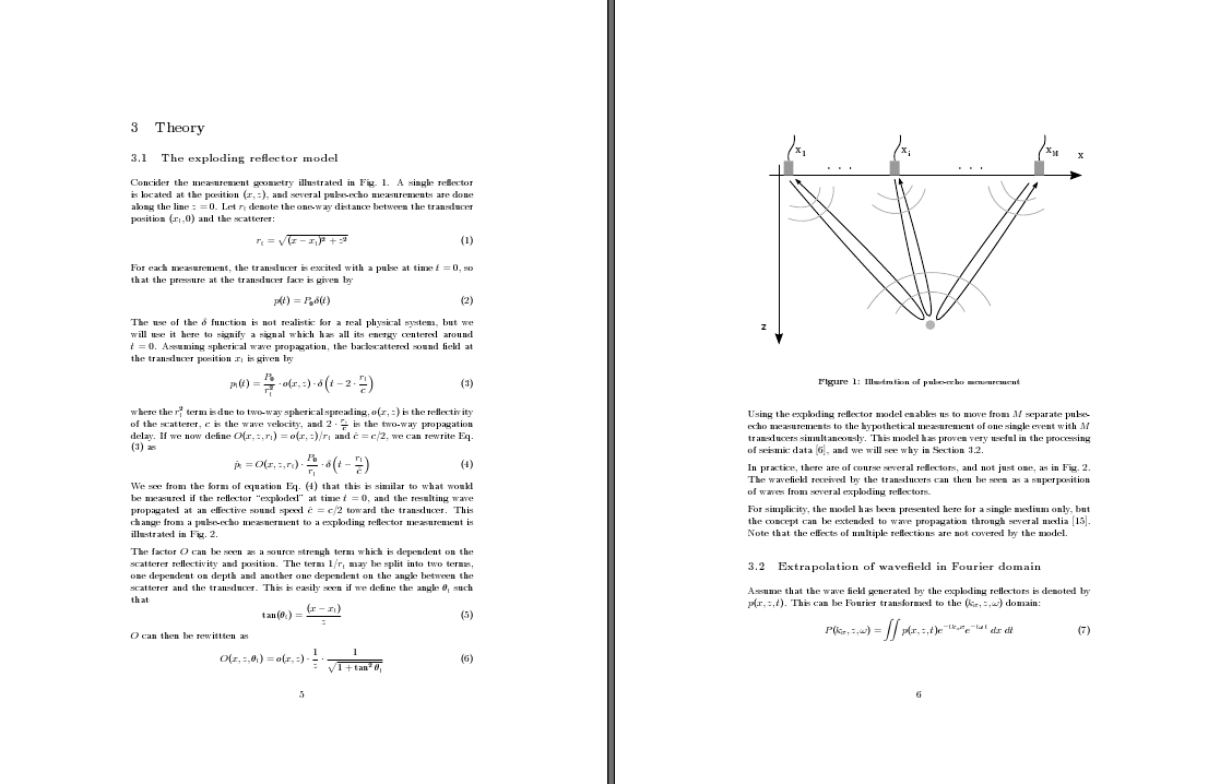
The default layout for an article in LaTeX is single-column, with quite large margins. The large margins are quite sensible, as they narrow the width of the column to make it easier for the reader to jump from one line to the next. However, when I write articles, I often include a lot of equations and figures, and these tend to create a lot of white space. The result is a massive number of pages which each has relatively little content, as illustrated by this example:



Switching to two-column layout is surprisingly easy -- just add the "twocolumn" option when declaring the document type, for example:

\documentclass[10pt,twocolumn]{article}

For figures, it is also useful to specify the width of the figure relative to the column width, like this:

\includegraphics[width=0.9\columnwidth]{Figures/figure1}

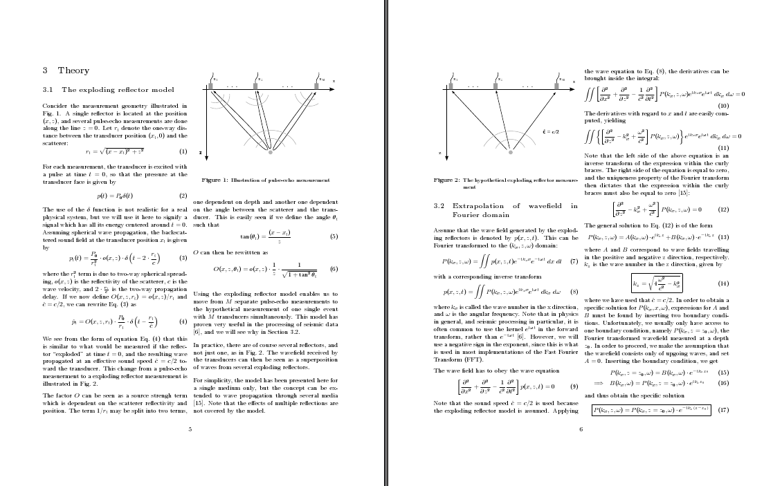
The result is a page with a lot mote information, which is also easier to read because of the columns are narrower than in the one-column layout. However, the pages also looks a bit crowded:



This is one of many cases where the geometry package comes in handy. Looking at the pages above, it seems that the separation between the columns is a bit too small, especially compared with the outer margins. We include the geometry package and increase both column separation and text width/height:

\usepackage[width = 18cm, height = 22cm, columnsep = 1cm]{geometry}

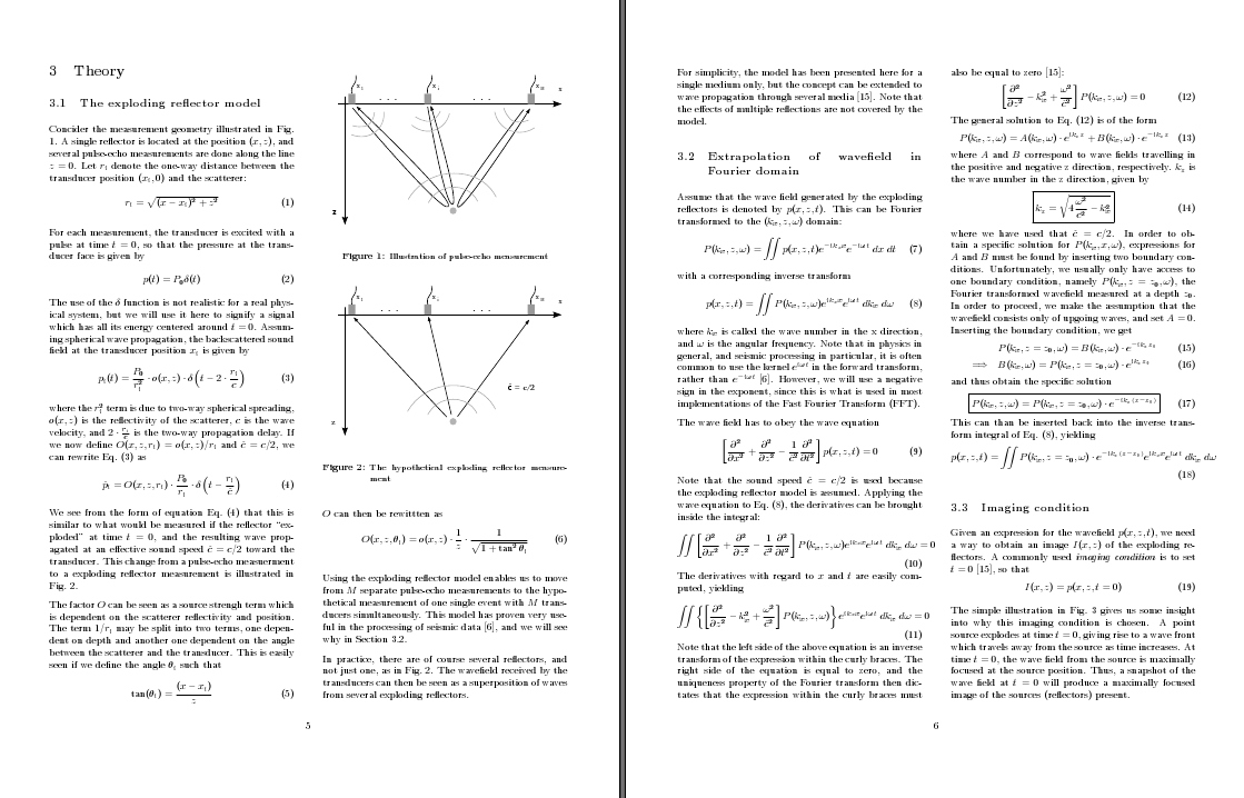
Note that these parameters are only a few of the parameters that can be set using the geometry package. Consult the documentation for further details. The end result is, in my opinion, quite pleasing compared with the initial one-column layout:



And, lastly, a small but useful detail: If you want a figure or table to span the width of both columns, add an asterisk when declaring the environment:

\begin{figure*}
...
\end{figure*}

If you found this interesting, check out Robert Felty's blog post on the same subject. Also, if you have any other tips concerning one-column versus two-column layouts - please share them here! :-)

Setting file permissions in linux

File permissions for a file or a directory are grouped after "user" (u), "group" (g) and "other" (o), and permission to read (r), write (w) and execute (x). In your home directory, you are registered as the user of all the files, and by default you have read, write and execute premission to all files.

The file permissions can be seen by typing "ls -l" in the terminal. The permissions are then listed as a string, for example "drwxr-xr-x". This string consists of a "d" plus three groups of "rwx", corresponding to the user, group and others, respectively. The "-" sign indicates "no permission". For the example above, the user has all permissions, while the group and others only have read and execute permissions.

File permissions are set by the "chmod" command. One way to use this command is to add (+) or remove (-) permissions. For example, the following command adds permission for user and group to write and execute "somefile.txt"


chmod ug+wx somefile.txt

The same syntax is used for files and folders. To set permissions for all files and subfolders of a folder, add a "-R" ("recursive") switch. For example,

chmod ugo-w -R SomeFolder

will remove all write permissions for "SomeFolder" and all its contents.

This approach is based on changing the file permissions relative to the way that they were before. The file permissions can also be set "absolutely". It is common to do this by coding r,w and x as numbers 4, 2, and 1. The file permission is then identified by the sum of the numbers, for example "r-x" = 4+1 = 5. For example, to let the user have all permissions while restricting write access for group and others, "rwxr-xr-x" can be translated to 755, and the chmod syntax is as follows:

chmod 755 file.txt

For further information on file permissions and how to change them, consult the Ubuntu Community Documentation.

The curse of Matlab NaNs

NaN is a special kind of Matlab value, representing Not-A-Number. This is often returned from a function or operation where the output is not well defined. For example, if you try to interpolate a value outside of the range of x values, the interp1 function returns NaN for this value. The following sample code illustrates this:

x = [1 2];
y = [1 4];
xi = 5;
y = interp1(x,y,xi)

returns y = NaN.

You may not always notice that a variable contains NaN values. For example, let's plot the "peaks" matrix from Matlab as an image:

X = peaks;
imagesc(X)



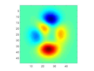
Now, if we set the middle element equal to NaN, this will show up as a blue spot in the image. This is because Matlab plots NaN elements with the "lowest" colormap color:

X(25,25) = NaN;
imagesc(X)
colorbar



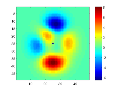
Note here that there is no way of distinguishing a NaN from a valid data value in such an image. However, we can check how many NaN elements there is in a variable:

numberOfNanElements = nnz(isnan(X))

which returns 1. Now, NaN has the unfortunate property that is "taints" all other elements that are affected by it. For example, if we take a 2D Fourier transform of X, all the elements returned by the function are NaN. So,

nnz(isnan(fft2(X)))

returns 2410! One single NaN pixel in the original image makes the entire transform unusable. Although I can understand the logic behind this behavior, it has been (and still is) a frequent source of very frustrating bugs in my work. When debugging, I often check 2D datasets by plotting them as images -- but as we have seen, a few NaN values can easily be present in an image without standing out from the valid data points. So, thinking that the dataset is valid, I continue stepping through the code, only to find that the complete dataset suddenly turns into NaNs. In this situation it is easy to conclude that there is something wrong in the last function used, when the fault really lies in the input data.

I've spent too many hours agonizing over such errors, so here's a tip for everyone that think that NaNs are messing up their code: For all variables that may potentially contain NaNs, set all NaN elements to zero, like this:

X(isnan(X)) = 0;

A zero value may not necessarily be "correct" as such, but it doesn't have the potential of NaNs to destroy the complete dataset. Now, if I could only remember this the next time I encounter "the curse of the NaNs"... ;-)

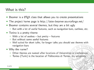
Introduction to Beamer presentations

I just started using Beamer, which is a document class for creating presentations using LaTeX. I installed Beamer in Ubuntu Linux using the Synaptic package manager, and found the user guide located in /usr/share/doc/latex-beamer, along with a set of useful templates. The user guide is massive and although it probably contains everything there is to know about Beamer, I searched the web for some quick introdutions:

A Beamer Quickstart is a very good starting point for Beamer - it both contains the essential "hello world" code for a bare-bones presentation, plus a lot of details on how to customize your presentation.

Sylvia Blaho at my very own University of Tromsø has also made a nice introduction to Beamer, as a Beamer presentation, of course.

Beamer comes with a set of themes and color layouts, and this Beamer Theme Matrix shows examples of every possible combination of these. Very useful for finding your favorite theme. Note that the .sty files for all the themes are located in /usr/share/texmf/tex/latex/beamer/themes.

There are also a lot of people making their own Beamer themes. This webpage has a list of several such themes made, among them the beautiful Torino theme and an unoffcial but really nice theme for Uppsala University.

Problem loading Ubuntu 9.10 (Wubi) after update

Today I installed an Ubuntu update and rebooted the machine, only to find that I was unable to start Ubuntu. In stead, I was stuck within the "GRUB boot loader". After some intense frustration, followed by some grumbling research on another machine, I found the cause of the problem.

When I installed Ubuntu, I used Wubi, which installs Ubuntu as a Windows program. Wubi uses the GRUB boot loader, but there is a bug in GRUB which can potentially disrupt the Ubuntu boot process each time the linux kernel or GRUB is updated. The problem and its solution is described on this Sourceforge wiki page. In short, one needs to log into windows and replace the faulty file wubildr in the C:/ folder with this file.

Matlab figure with zoomed-in plot of area of interest

I came upon a Matlab file at the File Exchange website which lets you add additional subplots of zoomed-in areas in the figure. This looks hugely useful, for example for magnifying details on an image while still seeing "the big picture".

Changing text size in LaTeX

One of the advantages with LaTeX is that you don't really have to worry about font sizes, heading layout etc. - you can just structure your document, and the LaTeX compiler will take care of the rest. You can of course set the "global" font size when declaring the document class, for example

\documentclass[10pt]{article}

However, sometimes you want to change the relative size of some block of text. To do that, use the following syntax:

{\textsize Text with different relative size}

where you can replace \textsize with any of the following sizes:

\tiny \scriptsize \footnotesize \small \normalsize
\large \Large \LARGE \huge \Huge

Jagged text and graphics for scanned PDF documents in Ubuntu

I download a lot of scanned articles in my work. These are usually in PDF format, and the default viewer for PDF files in Ubuntu is Evince. However, for the scanned articles, the text is really jagged and hard to read. It seems that this is due to "missing anti-aliasing", and judging from this forum thread, several other users are having the same problem. A fix seems to be on its way, but while I'm waiting, I've installed Okular (a document reader for the KDE desktop), which renders the scanned text beautifully.

Comparing files in Ubuntu (graphical diff tool)

Today I found myself needing to compare two LaTeX files. I do my LaTeX editing in gedit, and was hoping that there might be a built-in diff tool. This is not the case (at least not yet), but after a bit of searching I found these programs:

• Meld, for the GNOME desktop
• KDiff, for the KDE desktop

Both programs can be downloaded from the Ubuntu repository (I was able to download it using the Ubuntu Download Centre), and both are able to compare and merge files and/or directories.

Note: There is also a command line diff tool (try diff --help), but I prefer a graphical interface for comparing files.

Compiling LaTeX code online

Have you ever needed to make a LaTeX document, without having access to a computer with a latex compiler? My wife had this problem today, and she emailed me and asked me to do the compilation. Of course some things had to be corrected, and we had to do a few email iterations before she was satisfied. Afterwards I started thinking that this must be quite a common problem, and that surely there must be some online service for compiling LaTeX code. And there is!

• This one has quite a nice GUI, and the possibility to output the compiled document in several different formats (PDF, PNG, etc.)
• This one is a lot simpler, but also works perfectly well.
  

Installing Octave on Mac OS X

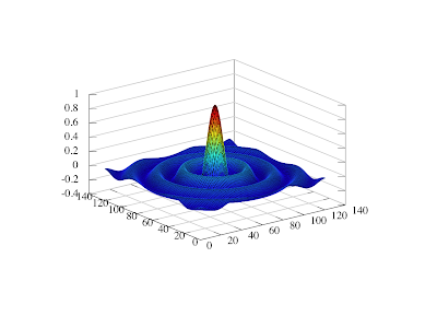
GNU Octave is a freeware alternative to Matlab which I have been curious about for some time now. I decided to try it out on my iMac, and downloaded it from Octave-Forge. At its core, Octave is a command-line program, but it uses GNUPlot for plotting figures. However, having installed both, I found that entering commands like

figure

or

plot(x,y)

had no effect at all. It seems that in order to work on Mac OS X, these two programs shuld be "glued together" by a third program called AquaTerm, which can be downloaded here. Having installed this, I am now able to make plots like the one below. Nice, eh? :-)

LaTeX in Blogger / Blogspot

UPDATE, 2012-02-13: The approach described under is now outdated. I would recommend taking a look at other alternatives, for example MathJax.

I was wondering if it would be possible to display latex formulas in Blogger - and of course it is. :-) I found a post by Watchmath describing how this can be done by adding a HTML/Javascript Gadget (like the "Blog Archive" on the right) with a little piece of javascript code. If it works, the following code

X(k) = \sum\limits_{i=0}^{N-1}x(n)e^{-2\pi ik \frac{n}{N}}

should magically turn into a beautiful LaTeX equation:

\[X(k) = \sum\limits_{i=0}^{N-1}x(n)e^{-2\pi ik \frac{n}{N}}\]

Nice! What's actually happening here is that the LaTeX expression is sent to a server for compilation, and then returned as an image which is pasted into the blog post. If you want to do the same, get the code and instructions here.

Note: This option does not work with "Preview" while editing - the code is compiled when the post is published, not before.

Browsing files in Ubuntu with superuser / root status

The file browser in Ubuntu is called Nautilus, and it works just like the Windows Explorer or Mac Finder. However, using Nautilus, I found that I was only able to move and delete files and folders within my home folder. To do anything outside this folder, I need "superuser" status. In the terminal, this "create folder"operation will not work:

mkdir /usr/share/newfolder

because I don't have write access to /usr/share. However, if I use "sudo" before the command, like this;

sudo mkdir /usr/share/newfolder

I am prompted for my password, and after entering it, I get superuser status and the folder is created. This works well for manipulating files and folders from the terminal, but I want to do the same using the graphical file browser Nautilus. The solution? Create a launcher on the desktop with the command

gksudo nautilus

gksudo is similar to sudo, but is used for graphical applications, as explained here. A window will pop up, asking for the password, and after entering it, Nautilus opens with superuser status.

Implementing linear interpolation for arrays

Here is a problem I recently came across in my work. How do you implement linear interpolation for arrays, and what is the corresponding computational complexity? I will come back to exactly what I mean by interpolation for arrays, but first, consider the image on the right.

We have two known points, (x1,y1), and (x2,y2), and we want to calculate the linearly interpolated value yi, given the x value xi lying between x1 and x2. The steepness of the line between the two points is given by a = (y2-y1)/(x2-x1), and yi can be expressed as yi = y1 + a*(xi-x1).

Assume now that we have an array x = [0 1 2 3 4 5] with a set of corresponding y values, and an array xi = [1.5 3.1 3.7] that we want to interpolate for. How can the above linear interpolation be implemented effectively for such arrays? Although the calculation of yi is easy enough, we first need to find (x1,y1) and (x2,y2) to be able to do it. After studying the Matlab function interp1q, I think I have some idea about how this may be done.

Let us take a simple example, where x = [0 1 2 3 4 5] and xi = [1.5 3.1 3.7]. We stack these arrays on top of each other, and sort them:

[xSorted,sortInd] = sort([x;xi])

yielding xSorted = [0 1 1.5 2 3 3.1 3.7 4 5], and sortInd = [1 2 7 3 4 8 9 5 6]. The values 1-6 in sortInd correspond to x, while the values 7-9 correspond to xi. Now, to interpolate, we want to know x1 x value that precedes each xi value. In the example above we can see that these values are [1 3 3], but how can we calculate them automatically?

We start by creating an index, called r, of which place the numbers in sortInd have in the array. This can be done in a for loop,

for ii = 1:length(sortInd)
r(sortInd(ii)) = ii;
end

but this operation can also be vectorized, using the (slightly confusing) Matlab statement

r(sortInd) = 1:length(sortInd)

which yields r = [1 2 4 5 8 9 3 6 7]. Compare this now with xSorted = [0 1 1.5 2 3 3.1 3.7 4 5]. Note that the three last values of r, [3 6 7], represent the position of the xi values in xSorted. We call these values ri, and "cut them out" by the following statement

ri = r((length(x)+1):end)

Now, let us take a look at which x values precede each xi value. For xi(1), 1.5, the preceding x value is given by x(2) = x(ri(1)-1) = 1. For xi(2), 3.1, the preceding value is given by x(4) = x(ri(2)-2) = 3, and for xi(3), the preceding value is given by x(4) = x(ri(3)-3) = 3. Thus, we see a pattern emerging here. The index for the preceding x value for xi(ii) is given by ri(ii)-ii. We call the index for the preceding x values pInd. They can be computed in a for loop,

for ii = 1:length(ri)
xpInd(ii) = ri(ii)-ii;
end

or, equvivalently,

pInd = ri-(1:length(ri));

yielding pInd = [1 3 3]. Using this, we can calculate the interpolated y values with the following statement:

a = (y(pInd+1)-y(pInd)) ./ (x(pInd+1)-x(pInd));
yi = y(pInd) + a.*(xi-x(pInd));

To summarize, the interpolation algorithm can be executed as follows

[xSorted,sortInd] = sort([x;xi]);
r(sortInd) = 1:length(sortInd);
ri = r((length(x)+1):end);
pInd = ri-(1:length(ri));

a = (y(pInd+1)-y(pInd)) ./ (x(pInd+1)-x(pInd));
yi = y(pInd) + a.*(xi-x(pInd));

My main reason for explaining this to myself was that I wanted to have some estimate of the algorithmic complexity of this kind of linear interpolation. The most computationally demanding operation in this algorithm is the sort. If N = length(x) and M = length(xi), the computational complexity of the sorting algorithm (and thus also the linear interpolation) is O[(N+M) log (N+M)].

UPDATE (2010-04-16):
I came across this post on linear interpolation on the MathWorks blog "Loren on the art of Matlab". It has a good explanation of the "binning" necessary to do the interpolation, plus a load of interesting comments / replies.

Installing Spotify on Ubuntu

OK, maybe Spotify isn't a "tool" as such, but it was nevertheless one of the first programs I tried to install on my new Ubuntu OS. There is no Spotify application directly available to Linux users, but it is possible to use the Windows application through a Windows emulator called Wine. With Wine installed, Windows programs can be installed and used in Ubuntu, without having to install a complete "guest" Windows OS (as you would do with e.g. VirtualBox).

Installing Spotify under Wine was really easy, but when I tried to run it, the sound was kind of distorted, and it would only play one song and then freeze. It turns out that this is a common problem in Ubuntu 9.10. Luckily, someone has already fixed it! This post on Jens' codelog describes what to do. In short, I had to uninstall Wine and install a new, modified version made by Neil Wilson. Now Spotify works like a charm, finally bringing some music into my office. Great!

A litte detail: There are no shortcuts or icons automatically created for Spotify. To create a shortcut on the desktop, right-click on the desktop and choose "create launcher". If you want a "proper" Spotify icon, you can use this SVG file created by Kalle Persson.

You can find more information on how to install and use Wine at this Ubuntu documentation page. There is also some more information on using Spotify under Wine on this Spotify FAQ.

Switching to Linux

As a first short post, I'll just mention that I recently installed Linux (Ubuntu) on my work laptop (a ThinkPad T61). Up 'till now, I've been using Windows XP (work policy), but I have been curious about Linux for some time now, and wanted to give it a try. Seeing as I also constantly have to deal with servers running on Linux anyway, I saw this as a nice opportunity to learn something new.

I always assumed that in order to install a second operating system, a second partition on the hard drive would also be needed. I was pleasantly surprised to find that Ubuntu can actually be installed as a Windows application. That's right, a whole operating system can be downloaded and installed as a regular application, and if you don't like it, you can also uninstall it as an application. In stead of using a separate partition, the Ubuntu operation system is saved in one big file, which works as a separate disk/partition when you are inside Ubuntu. The Windows installer can be downloaded here.

After installing, I restarted my machine, and a "boot loader" pops up, asking if I wanted to use Windows or Ubuntu. Choosing Ubuntu, I was amazed at how fast the startup process was (20-30 seconds), and having logged in, I found a beautiful, responsive GUI with a very nice selection of preinstalled programs. Everything worked "out of the box", and I was connected to the internet (wifi) and surfing within half a minute.

This "Ubuntu Windows Application" is highly recommended for anyone curious about Linux. I will keep posting my experiences with it as I go.