Implementing linear interpolation for arrays

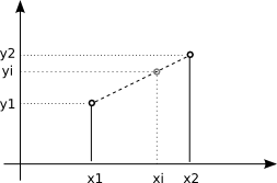
Here is a problem I recently came across in my work. How do you implement linear interpolation for arrays, and what is the corresponding computational complexity? I will come back to exactly what I mean by interpolation for arrays, but first, consider the image on the right.

We have two known points, (x1,y1), and (x2,y2), and we want to calculate the linearly interpolated value yi, given the x value xi lying between x1 and x2. The steepness of the line between the two points is given by a = (y2-y1)/(x2-x1), and yi can be expressed as yi = y1 + a*(xi-x1).

Assume now that we have an array x = [0 1 2 3 4 5] with a set of corresponding y values, and an array xi = [1.5 3.1 3.7] that we want to interpolate for. How can the above linear interpolation be implemented effectively for such arrays? Although the calculation of yi is easy enough, we first need to find (x1,y1) and (x2,y2) to be able to do it. After studying the Matlab function interp1q, I think I have some idea about how this may be done.

Let us take a simple example, where x = [0 1 2 3 4 5] and xi = [1.5 3.1 3.7]. We stack these arrays on top of each other, and sort them:

[xSorted,sortInd] = sort([x;xi])

yielding xSorted = [0 1 1.5 2 3 3.1 3.7 4 5], and sortInd = [1 2 7 3 4 8 9 5 6]. The values 1-6 in sortInd correspond to x, while the values 7-9 correspond to xi. Now, to interpolate, we want to know x1 x value that precedes each xi value. In the example above we can see that these values are [1 3 3], but how can we calculate them automatically?

We start by creating an index, called r, of which place the numbers in sortInd have in the array. This can be done in a for loop,

for ii = 1:length(sortInd)
r(sortInd(ii)) = ii;
end

but this operation can also be vectorized, using the (slightly confusing) Matlab statement

r(sortInd) = 1:length(sortInd)

which yields r = [1 2 4 5 8 9 3 6 7]. Compare this now with xSorted = [0 1 1.5 2 3 3.1 3.7 4 5]. Note that the three last values of r, [3 6 7], represent the position of the xi values in xSorted. We call these values ri, and "cut them out" by the following statement

ri = r((length(x)+1):end)

Now, let us take a look at which x values precede each xi value. For xi(1), 1.5, the preceding x value is given by x(2) = x(ri(1)-1) = 1. For xi(2), 3.1, the preceding value is given by x(4) = x(ri(2)-2) = 3, and for xi(3), the preceding value is given by x(4) = x(ri(3)-3) = 3. Thus, we see a pattern emerging here. The index for the preceding x value for xi(ii) is given by ri(ii)-ii. We call the index for the preceding x values pInd. They can be computed in a for loop,

for ii = 1:length(ri)
xpInd(ii) = ri(ii)-ii;
end

or, equvivalently,

pInd = ri-(1:length(ri));

yielding pInd = [1 3 3]. Using this, we can calculate the interpolated y values with the following statement:

a = (y(pInd+1)-y(pInd)) ./ (x(pInd+1)-x(pInd));
yi = y(pInd) + a.*(xi-x(pInd));

To summarize, the interpolation algorithm can be executed as follows

[xSorted,sortInd] = sort([x;xi]);
r(sortInd) = 1:length(sortInd);
ri = r((length(x)+1):end);
pInd = ri-(1:length(ri));

a = (y(pInd+1)-y(pInd)) ./ (x(pInd+1)-x(pInd));
yi = y(pInd) + a.*(xi-x(pInd));

My main reason for explaining this to myself was that I wanted to have some estimate of the algorithmic complexity of this kind of linear interpolation. The most computationally demanding operation in this algorithm is the sort. If N = length(x) and M = length(xi), the computational complexity of the sorting algorithm (and thus also the linear interpolation) is O[(N+M) log (N+M)].

UPDATE (2010-04-16):
I came across this post on linear interpolation on the MathWorks blog "Loren on the art of Matlab". It has a good explanation of the "binning" necessary to do the interpolation, plus a load of interesting comments / replies.